Table of contents:
Introduction
Branching
Result:
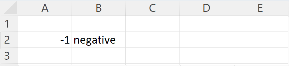
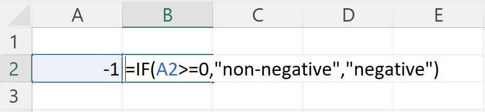
In some cases, we attach the operation to be performed to some conditions. We can use the IF() function to test a condition and determine what should happen if the condition is true and what should happen if the condition is false. Using the function:
- IF(condition; value_if_true; value_if_false)
- condition:
- here you must write a formula whose value can be true or false. You can refer to a cell (e.g. B3) or use some kind of comparison (e.g. B3>2 or B3=2).
- value_if_true:
- here we have to specify which operation the program should perform if the result of the above condition is "true". This can be a function (e.g. sum(B2:B5)) or text, number.
- value_if_false:
- here we have to specify which operation the program should perform if the result of the above condition is "false".
HINT: Excel can also interpret numbers as true/false values. If a number is non-zero, it is "true", if it is zero, it is "false".
Conditional aggregation
Most branching problems can be solved by using the IF() formula, as it can be freely combined with other functions. However, there are special cases that may be needed so often that there is a separate Excel function for them. These are conditional aggregation formulas, such as the COUNTIF() formula. The formula counts the number of cells in the selected range for which the condition is true. Usage:
- COUNTIF(range; condition)
- range:
- the cells in which we check whether the condition is met
- condition:
- a formula whose value can be true or false
Other conditional aggregation formulas:
- SUMIF(): sums the contents of the cells in the range for which the condition is met
- AVERAGEIF(): averages the contents of the cells in the range for which the condition is met
- SUMIF(test_range; condition; [summary_range])
- test range:
- the cells in which we check whether the condition is met
- conditions:
- a formula whose value can be true or false
- summary range:
- the cells whose contents we want to add if the condition is true in the given row of the test_range
HINT: If an input parameter to the formula is enclosed in square brackets, it is only optional to specify.
Naming the range
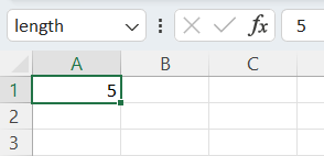
For complex formulas, it is more transparent to use unique names for the ranges rather than the default cell names. We can name a cell (e.g. "length" instead of "A1") or a range (e.g. "units" instead of "B2:B10"). To name it, we need to rename the cell name in the name field to the name of our choice. Names can be deleted/modified in the Formulas / Name manager menu.
HINT: If we refer to a range/cell by a unique name, Excel automatically treats it as an absolute reference.
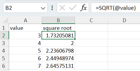
We can also name a whole column. Click on the column header to select the entire column and change the name in the name field (e.g. from "A:A" to "value"). If you then want to use a formula that refers to an element in the given row of column A, you must put an @ sign in front of the column name. Thus @value in cell B2 refers to cell A2, in cell B3 to cell A3 and so on.
Quadratic equation
Exercise: write the solutions of the quadratic equation ax² + bx + c = 0 depending on the parameters a, b, c. If there is no solution in the set of real numbers, write "the discriminant is negative"!
Solving formula of the quadratic equation ax² + bx + c = 0:
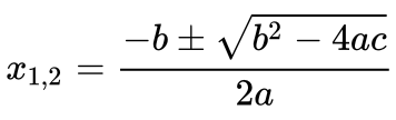 ,
and the discriminant is the part below the root. If the discriminant is negative, then there is no solution to the equation on the set of real numbers.
,
and the discriminant is the part below the root. If the discriminant is negative, then there is no solution to the equation on the set of real numbers.
First, let's create the parameters and name the cells so that we can easily refer to them in the formulas.
- Enter "a", "b", "c" in cells A1, A2, A3.
- Then enter any numbers you like in cells B1, B2, B3.
- Let's name cells B1, B2, B3 a, b, cc. (The name c is unfortunately already taken by default.)
Let's calculate the discriminant and check if it is negative.
- Write "D" in cell A5.
- Calculate the value of the discriminant in cell B5, using the unique names:
=b^2-4*a*cc - Name cell B5 D.
- Check in cell C6 whether the discriminant is negative:
=IF(D>=0; "non-negative"; "negative")
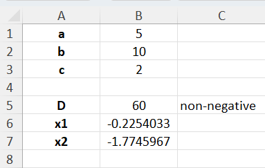
- Write "x1", "x2" in cells A6, A7.
- In cell B6 enter the solver formula:
=IF(D>=0;(-b+sqrt(D))/(2*a); "negative discriminant") - In cell B7 enter the solver formula:
=IF(D>=0;(-b-sqrt(D))/(2*a); "negative discriminant")
HINT: If you want nothing at all in the cell, replace "negative discriminant" with "".
Cost plan for a building under design

Excercise: a large building is in the planning stage. Unfortunately, not much is known about the plan, not even the ceiling height, but we know that the rooms are rectangular. When the plans are finalised, you will receive a .csv file with the room details (room name, length, width, flooring). You will then have to answer the following questions in a very short time:
- how many m² of each type of flooring are needed?
- in total, how much does each type of flooring cost?
- how many rooms are covered by each type of flooring?
- how many m² should be painted?
Prepare a spreadsheet so that when you receive the data and find out exactly which floorings and paints will be planned (and this may change later), you can quickly enter them and calculate the requested data.
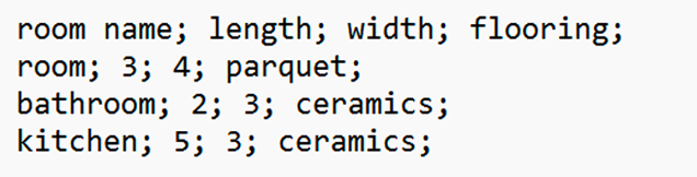
We can easily read the .csv file with Excel. If the data is received in the format shown in the illustration, each row will have a room and four columns: room name, length, width, flooring. Let's first create the location of these data and enter any data we like, so that we have something to work with.
- Enter the headers in cells A1:D1 and enter 2-3 lines of data.
- Name column B as "length", column C as "width" and column D as "flooring".
- In cells E1, F1 enter the terms "floor area", "surface to be painted".
- Let's name column E "floor_area".
HINT: If the naming failed because we accidentally named the wrong range, we can delete the wrong name in Formulas / Name manager.
- In cell H1 we write "ceiling height".
- In cell I1, enter an arbitrary number (e.g. 2.65) and name the cell "ch".
- In cell E2, calculate the floor area using length and width:
=@length*@width - The surface to be painted is the floor area + perimeter*ceiling height. Calculate this in cell F2:
=(@length+@width)*2*ch + @floor_area
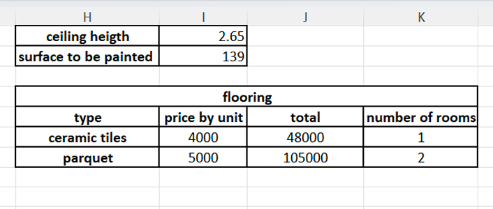
- In cell H2 write "surface to be painted" and in cell I2 calculate its value:
=sum(F:F) - Underneath, make a small table as shown in the illustration.
- Enter random unit prices in cells I6, I7 (we don't know the exact values yet).
- Calculate the cost (price per unit * total area) for the first cover. For the total area, we use a conditional summation, as we only want to sum the area of the rooms where the flooring is installed:
=I6*SUMIF(flooring;H6;floor_area) - For the first cover, calculate how many rooms it is in!
=COUNTIF(flooring;H6) - Copy the formulas by dragging down.
Filtering and sorting data

Excercise: the building plan discussed in the previous exercise has been completed, and the data is available in the helyiseglista.csv file. The ceiling height is 3m, and we have to estimate the prices. We need to take the spreadsheet to a consultation, where we need to be able to quickly answer questions such as:
- Which room is the biggest?
- Show me a list of rooms with parquet flooring!
- Show a list of rooms over 30m²!
- Let's look at the rooms by flooring, in ascending order of floor area!
Prepare for the consultation. Import the data you created in the previous exercise, then use a filter and perform the queries above.
First delete the randomly entered data and fill it in with the correct values.
- Go to File/Open/Browse menu, choose "All files" and select the csv file. In the settings, select that the data is separated by semicolons.
- Copy the data into the corresponding cells of the already prepared table.
- Correct the ceiling height to 3m.
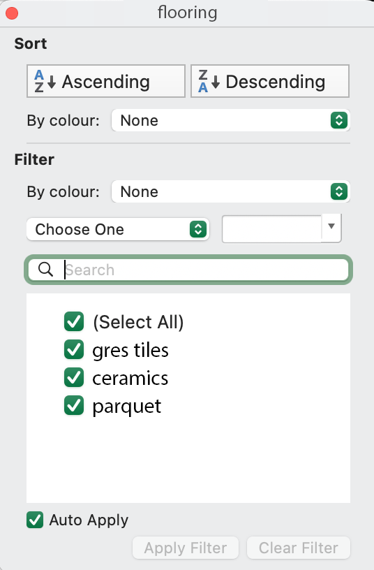
In the small tables on the right about pavements, the names of the pavements should be corrected. Let's turn on the filter to see how many different floorings there are.
- Click into the table containing the data (e.g. cell B3).
- In the Home / Sort&Filter menu turn on the
 filter. Small arrows will then appear next to the names in the header of the table containing the data.
 - Click on the small arrow in the flooring column to see the options. This will show you all the different floorings.
- Correct the list of floorings: delete the old floorings and enter the correct values.
- Search online for the price of each type of flooring, choose one and enter the price in the table
You can compare your solution with the solution key.
Use the filter to answer the questions above.
- To find the largest room, sort the rooms by floor area in descending order using the the filer of the floor area column.
- If you only want to see the rooms with parquet flooring, you need to remove the tick from the other flooring types in the filter.
- For rooms with a floor area greater than 30m², select "Greater than" from the drop-down menu in the floor area filter and enter 30 in the box next to it.
- Remove all filters and sort the table first by floor area and then by flooring using the filter.
Note: For more complex tables, for buildings with hundreds of rooms, the above solution is slow, with many possibilities for error. Dynamic formulas can be used to solve similar problems more efficiently. The dynamic formulas are part of the subject materials of the subject Digital Representation